

The APH campaign is a good case study for the Fibonacci Scale SystemTM for a couple of reasons: 1) It illustrates many of the mechanics of the system and 2) highlights the power of the system applied to return on capital employed (ROCE). This article will walk through the campaign in the context of any trading system.
1. Defined Universe Selection
A strategy must clearly define what it trades.
In July I published a piece titled Scale Trading Edge: Wide Moat Dividend Paying Stocks discussing why institution grade equities are perforce for scale trading. The main points being that these stocks are:
· Liquid
· They are not likely to go to zero
· They pay you to wait
· You can start small.
Read the full article at Scale Trading Edge: Wide Moat Dividend Paying Stocks. These stocks are the universe from which all campaigns are initiated. We will also periodically use an ETF or a stock that may not have a wide moat but at least a narrow moat and some other competitive advantage.
For this trade our wide moat dividend paying stock is Amphenol ticker APH.
2. Entry Rules (The Setup)
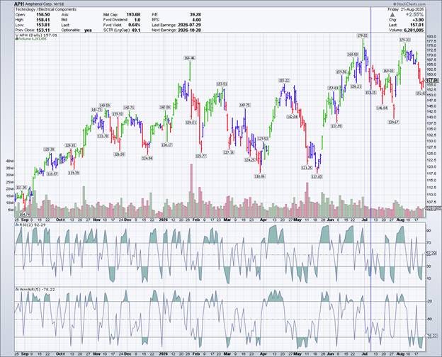
For the Fibonacci Scale SystemTM we find a wide-moat-dividend paying stock that is suffering some type of pullback. As you can see from the chart, on 7/8/2026 (vertical blue line) APH was oversold according to both the RSI(2) and Williams %R (5). This was our entry signal. We entered on the afternoon of 7/8/2026 at a price of 156.90.
3. Position Sizing & Capital Allocation
Position sizing determines survival. A great setup with poor sizing will eventually blow up an account.
Unit Sizing: The exact dollar amount or percentage allocated to the initial tier. For our public account we are using a $1,000 dollar starting unit. This would be 2% of a $50,000 dollar account. There will be more in-depth articles on position sizing but for this campaign the unit size is $1,000.
Scaling Rules: We added/subtracted capital using the Fibonacci sequence for both the number of units per layer and distance that layer was from an anchor. Since our entry was 156.90, we rounded the anchor to 157.00. For the depth of the scaling tiers, we used 2%. More in-depth discussion on depth selection will also be covered in future articles. For this trade, however, just know the width was 2%.
Risk Per Trade: We cap the maximum allowable loss on a single campaign to a defined fraction of total portfolio equity which is 2% of portfolio equity, or $1,000 for this $50,000 account.
Scale Grid: Below is the final scale grid:

This is the buy/sell roadmap for the rest of this campaign. We will discuss in detail how to use the road map in future articles. For now, just note this is the grip we used for this campaign.
4. Exit Architecture
A complete strategy always knows how it will leave a position before entering it.
Profit Taking / Trend Capture: Our objective with this strategy is to scale in an out until our campaign cost is below a swing low then shift to a trend following indicator as a stop loss.
Loss Mitigation / Invalidation: Our loss mitigation is a $1,000 loss on the campaign.
Below is the trade history for the campaign.

We began the trade on 7/8/2026. Our unit size of $1,000 rounded to 6 shares for our initial purchase at 156.90. If you refer back to the chart you will see that APH caught a slight move up, then hovered around our entry for a few sessions. On 7/16 we picked up 7 shares at 153.75 then on the next day we picked up 14 shares at 147.50. Notice the 1,1,2 pattern. In this case the 14 shares bought at the 2-unit level was as deep as this trade went into the scale. On the same day we sold 7 of those 14 shares at 152.56. Note for scaling out we invert the sequence and scale out from the last layer at a 1,1,2 rate as well.
Between 7/20 and 7/30 we rocked back and forth buying and selling 7 shares at a time, all the while reducing our average campaign cost. By the end of the day on 7/30 we had sold all but the 6 shares we began with but now our average cost for the campaign applied to those shares is 98.71.
As you will see in the chart below, the swing low at that time was 139.67. We chose to use the Parabolic Stop and Reverse as our trailing stop. The overlay has been added.
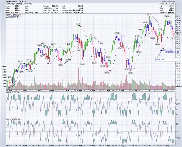
Once we moved into trend mode, we ceased any scaling back and forth and strictly followed the trend until we were stopped out at 163.03 on 8/18/2026. Our average cost for the campaign applied to those final 6 shares was 98.71. We were stopped at 163.05 for a profit of 397.94. Below is a summary of the ROCE.

As you will see in the in the figure detailing each trade the capital employed is weighted on a daily basis then totaled and divided by the number of days in the trade to get the actual ROCE. For this trade we picked up an annualized ROCE of 263.53%. While we didn’t have but a little over 2% of the account tied up in this campaign the return on that money was outstanding.
Summary
This was just a brief summary of how the Fibonacci Scale SystemTM works. As we move forward there will be future articles going in far more depth on the nuts and bolts of implementing the system. While there are a few moving parts, the system is robust and mathematically sound. We will be proving that over the next few months.