

I read a note from a respected poster last night that went something like this (I am paraphrasing)
“The reason to trade index funds is summed up in one sentence: 92% of professional money managers do not beat the index. Why do you think you can as an amateur?
It is a legitimate question and a clever soundbite. It sounds prudent, data-driven, and final. But it relies on a fundamental misunderstanding of portfolio theory and institutional reality: it confuses raw total return with risk-adjusted return.
When an amateur looks at an equity curve, they often ask only one question: “How much money did it make?”
When a professional risk manager or institutional allocator looks at that same curve, they ask a very different question: “How much risk did you take to generate that return?”
I’m not certain all those 92% of money managers that were not beating the S&P 500 were actually failing. My belief is many have managing mandates designed to avoid catastrophic drawdowns while seeking an adequate return on excess risk?
If you want to evaluate any trading strategy—whether an index fund, an active fund manager, or your own systematic framework—you need to look past nominal returns and understand one of the most important metric in quantitative finance: The Sharpe Ratio.
What Is the Sharpe Ratio and Who Uses It?
Developed by Nobel laureate William F. Sharpe in 1966, the Sharpe Ratio measures the excess return of an investment asset or portfolio above the risk-free rate, divided by its standard deviation (volatility).
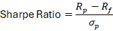
R p= Expected Portfolio Return
R f= Risk-Free Rate (e.g., short-term US Treasury Bills)
σp= Standard Deviation of Portfolio Excess Return (Volatility)
In plain English: It tells you how many units of return you receive for every unit of volatility you endure.
How Institutional Allocators Interpret the Numbers:
< 0.50: Suboptimal / Poor. You are accepting substantial volatility without proportional compensation.
0.50 – 0.99: Acceptable / Average.
1.00 – 1.99: Good to Very Good. The gold standard threshold for systematic strategies.
≥ 2.00: Exceptional (rarely sustainable long-term without heavy structural edges).
Who Uses It and Why?
Pension funds, sovereign wealth funds, hedge fund allocators, and family offices rarely hand capital to a manager based purely on double-digit annualized returns. If a fund returned 20% last year but suffered a 45% intra-year drawdown with wild volatility, its Sharpe ratio is poor. That manager is one market shock away from insolvency.
Institutions use the Sharpe Ratio to determine skill versus luck (leverage). Anyone can boost nominal returns by applying 3x leverage to the S&P 500, but leverage magnifies volatility at the exact same rate—leaving the Sharpe Ratio unchanged while dramatically increasing the risk of absolute ruin.
The S&P 500’s Secret: A Suboptimal Sharpe
Buy-and-hold indexing advocates present the S&P 500 as the ultimate investing vehicle. While the long term gains are most definitely positive when looking at those gains compared to risk, present another picture. Historically, the S&P 500 delivers an annualized Sharpe Ratio hovering around ~0.70 to 0.80 over long cycles (and significantly lower during secular bear markets or high-rate environments).
Why? Because 100% equity exposure subjects you to the full brunt of market variance:
Unmitigated Drawdowns: Market cycles routinely produce 20%, 30%, and 50% drawdowns (2000–2002, 2008, 2020, 2022).
Capital Inefficiency: To capture the index return, 100% of your capital must sit exposed to equity market beta 100% of the time.
A Sharpe of ~0.70 means passive equity investors are enduring significant volatility for an unoptimized return profile.
How to Improve Sharpe: Capital Efficiency & Asymmetric Allocation
There are mathematically two ways to engineer a Sharpe Ratio above 1.00:
Reduce Portfolio Volatility: Dampen drawdowns and portfolio variance.
Maximize Return on Invested Capital (ROIC) on Active Exposure: Generate high velocity and high return on a fraction of the total portfolio, while parking the remainder in risk-free or low-volatility yield instruments.
This brings us to how a quantitative, rule-based approach solves the indexer’s dilemma.
Engineering a >1.0 Sharpe: The Fibonacci Scale System™
The Fibonacci Scale System™ was designed from the ground up to address the structural inefficiencies of passive buy-and-hold investing.
Instead of deploying 100% of capital into market beta and riding drawdowns to the bottom, the system operates on a quantitative barbell framework:
TOTAL PORTFOLIO
Active Campaign Engine (Limits on total cash used for new and trend following campaigns)
Wide-Moat Dividend Stocks
Tiered Fibonacci Scaling (1, 1, 2, 3, 5, 8)
Beta Volatility Spacing
Trend Capture Exits (Donchian / SAR)
Risk-Free Portion
T-Bills / High-Yield Cash Equivalents
Zero Volatility Sleeve (σ = 0)
Dry Powder & Drawdown Protection (20% cash minimum)
Here is how the mechanics systematically compress the denominator (σ) while expanding the numerator (Rp-Rf ):
1. High Velocity on Employed Capital
The system does not commit 100% of portfolio capital to active risk. By deploying capital only into high-conviction, wide-moat, dividend-paying equities during defined pullback zones, then churning those stocks through the scaling tiers, the Return on Capital Employed (ROCE) on the active sleeve is high.
2. Scaling via Fibonacci Math (1, 1, 2, 3, 5, 8)
Rather than suffering standard equity drawdowns on a full, lump-sum position, initial exposure starts small (1 unit). If price pulls back through beta-based volatility tiers, the grid scales down in both unit size and spatial spacing.
The Math: Your average cost basis drops non-linearly toward the current market price. A minor structural rebound recovers the campaign to profitability without requiring the stock to reclaim its previous all-time high.
Once a scaling tier is initiated, scaling out of that tier generates “production” effectively lowering the average cost per share of the campaign.
3. The Baseline Yield Buffer
Because the system mandates a strict 50% cash floor circuit breaker for new campaigns, and caps total active deployment to leave at least 20% cash, a substantial portion of the portfolio sits in risk-free instruments (Treasury Bills / Cash Equivalents earning the prevailing risk-free rate).
This creates a volatility drag in reverse: the cash sleeve has near zero volatility, directly suppressing total portfolio standard deviation.
Meanwhile, active positions collect continuous dividend income, adding an incremental buffer to downside movement.
4. Asymmetric Exit Strategy (Transition to Trend Mode)
Once a campaign recovers through its scale tiers and production and establishes a campaign price below a risk a trailing stop, the system transitions to Trend Mode—locking in a now risk-free trailing stops (via indicators like the 10-day Donchian Channel or Parabolic SAR) to let winners run. Once in trend mode no more purchases or scales are made. We scaled into pullbacks with mathematical edge and now we will ride a risk free trade with trend following mechanics.
The Bottom Line
When someone asks, “Why do you think you can beat the 92% of money managers?”, the answer is: I don’t.
The answer is that you are not playing the nominal return game—you are playing the risk-adjusted return game.
Passive indexing accepts 100% market variance for a 0.70 Sharpe. By being an active trader combining a structural risk-free cash base with mathematically scaled, high-ROIC active campaigns in wide-moat assets, a systematic framework, you can target an institutional-grade Sharpe Ratio (>1.0): providing adequate returns, minimal drawdowns, and structural peace of mind.
Data collection and forward-testing campaign logs are ongoing. Subscribe to follow the real-time campaign performance and mechanical breakdowns of the Fibonacci Scale System™.
Stay tuned!!
See trading journal at Public Trading Journal.xlsx